Economic Analysis on Gacha Game Pricing - Part 4 - Simulating Consumer Spending

Written by Researcher Alex and Edited by Rei Caldombra 12/8/25 Previous Part: Economic Analysis on Gacha Game Pricing - Part 3 - The Pricing of Gacha Games — Blog Under a Log

Consumers in free-to-play games such as gacha games need disposable income to pay for their paid rolls or chances to get a digital product in a free-to-play video game. However, their decision to spend on a digital product is tied to two key factors. The first factor is the fixed cost of hardware required to play the game whether that being a console, phone, or computer. The second factor is if there are other similar digital products in other games. Should the consumer spend their money in the free-to-play game to get a digital product or in another free-to-play game that has an identical digital product? We can calculate this in a simple formula where the digital product has the quality that the consumer desires:

Consumer will pay for a specific quality=((The total accumulated disposable income per consumer - initial fixed cost of hardware) * (a game that has preferred quality)) / (all other games with identical quality)

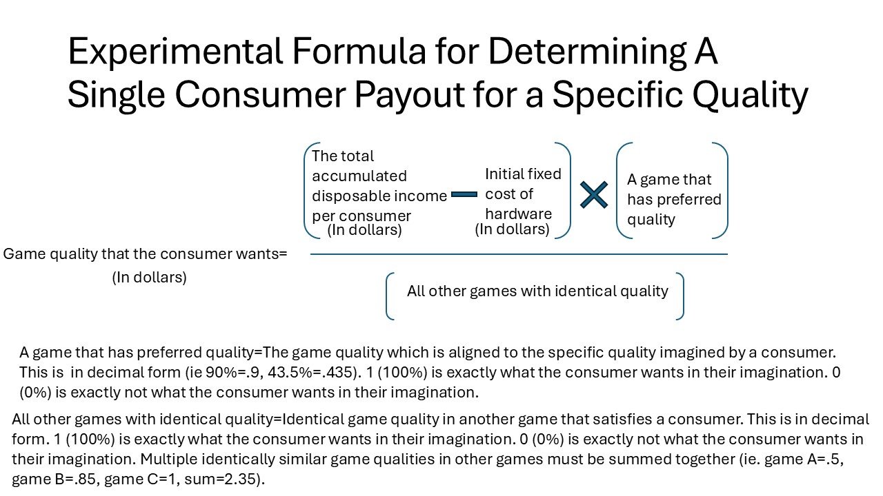
In this formula, the game quality that the consumer wants is how much the consumer is willing to pay for the specific quality that is in the digital product. This is represented in dollars. The total accumulated disposable income per consumer is the amount of money that the consumer is willing to spend in the game. This is subtracted by the initial fixed cost of hardware in dollars. This can be the cost of a phone or console to run the free-to-play game. This net value is then multiplied by how similar the game quality is to what the customer imagined. This is labeled as a game that has preferred quality in the formula. In short, a consumer would likely pay less if they get only what the consumer wanted to pay for and more if they get what the consumer exactly wanted. This is written in decimal form that represents a percent with 100% of what the consumer wanted being 1 while 0% of what the consumer wanted being 0. Using the same decimal form scale, all other games that have similar qualities are summed together. For instance, other game A has a quality that is 100% what a consumer wants and other game B has a quality that is 50% of what a consumer wants. This can be written as 1+0.5=1.5. This represents all other games that the consumer can choose instead of the game that has their specific quality. Finally, the net value which is multiplied by how aligned the quality of the game aligns with the consumer's imagination is then divided by the sum of all other similar qualities in other games. 

To show that this formula works, consider this example below:

So a consumer wants a specific quality of a plain circle pizza image in a free-to-play game and has $100 of disposable income. The consumer had to buy a cheap game console worth $50 to play the free-to-play game on it. In the free-to-play game, there is a digital product of a plain circle pizza image that is exactly 100% of what the consumer imagined.

Looking at other games, the consumer sees three games that have digital products with similar qualities. Game A has a digital product that is plain half circle pizza which is 50% of what the consumer wants in their imagination. Game B has a digital product that is plain circle pizza that has some toppings on it that take up 5% of the space on the pizza which is 95% of what the consumer wants in their imagination. Game C has a digital product that is plain circle pizza which is 100% of what the consumer wants in their imagination. These three other options are what the consumer can choose as an alternative to the digital product in the free-to-play game that the consumer is playing. This can be placed in the formula:

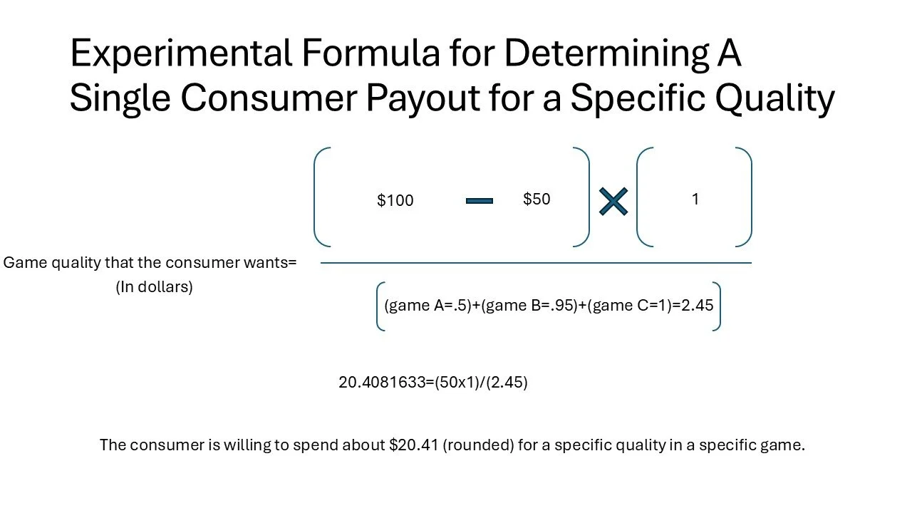
When calculated, the consumer is willing to spend about $20.41 for a specific quality of a plain circle pizza image in a free-to-play game.

This formula provides a simplified explanation for how much a single consumer could pay for a single quality in a specific game. In this case, this could serve as a derivative for each copy of a game bought by a consumer in a fixed sale or chance sale. Hypothetically, each consumer may have similar and different spending budgets which can be arranged on a graph to fit both fixed and chance saving graphs. In short, let's put a bunch of consumers with varying levels of spendable disposable income together as a consumer group.

This consumer group can be plotted out in a chart.

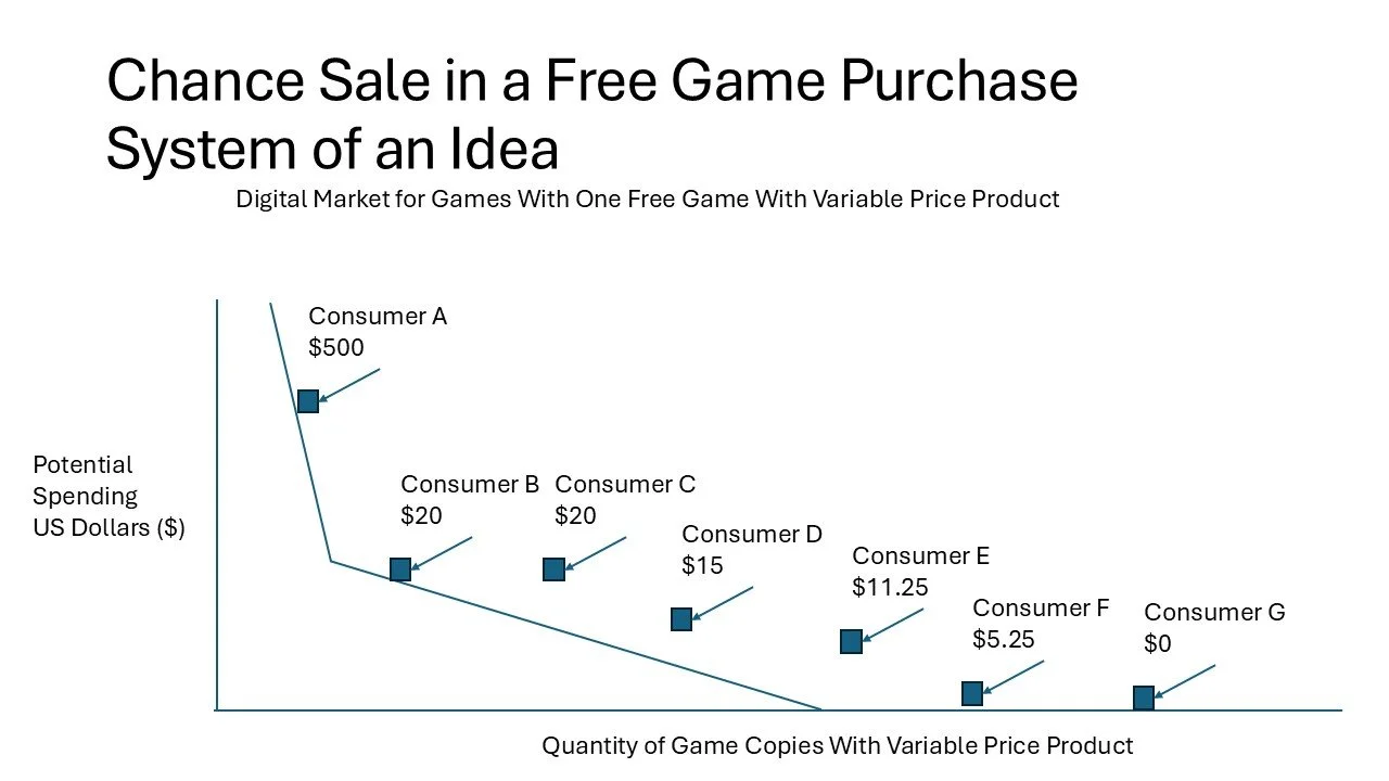
In this chart, the “Potential Spending US Dollars ($)” axis shows how much disposable income in US dollars a consumer may hold at a specific point in time. The “Quantity of Game Copies With Variable Price Product” axis which shows each consumer having a playable game that can sell the product to the consumer. The chance sale is the game company selling chances for a consumer to possibly get a product. This product is a variable price product because the product's worth is determined by the total chances bought by the consumer. In other words, a chance sale is just the selling of lottery tickets that could let a consumer win a product per each lottery ticket. The product's worth is decided by how many lottery tickets are bought which varies between each consumer.

Although this chart represents a chance sale such as a gacha mechanic in a game, it can also be used for selling a product at a fixed price. Simply drawing a horizontal line on the chart can show the price of the product. Anyone equal to and above the horizontal line would be able to purchase the product. In short, this chart is just for showing where the consumer is relative to other consumers based on their disposable income. Yet this chart can be used to show if a consumer can afford a fixed price or variable price product.

Now it is completely possible to calculate if consumers can afford a product. I have created a table below to show how this can be calculated.

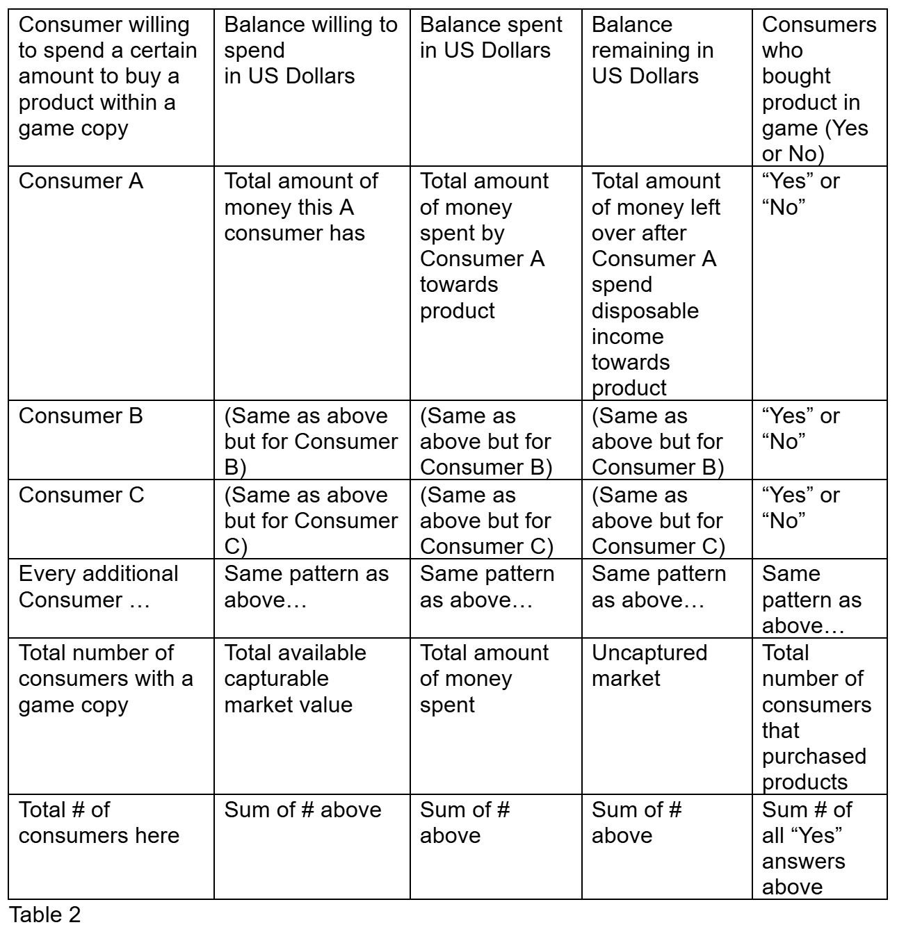
All this table does is show how much disposable income each consumer has, how much each consumer spent, and how much disposable income each consumer has after spending. The table sums all the disposable income, the spending, and the balance remaining after spending for all the consumers. Additionally, the total number of consumers that can afford the product and the total number of consumers that have the game is also listed in this table.

To demonstrate that this table works. Let’s sell a fixed price product like a digital lamp in a game at $13 to all the consumers in the graph.

As shown in this table, consumers had $571.50 of disposable income and could only spend $52. All 7 consumers had a game but only 4 people could buy the product. $519.50 still remains in the hands of consumers.

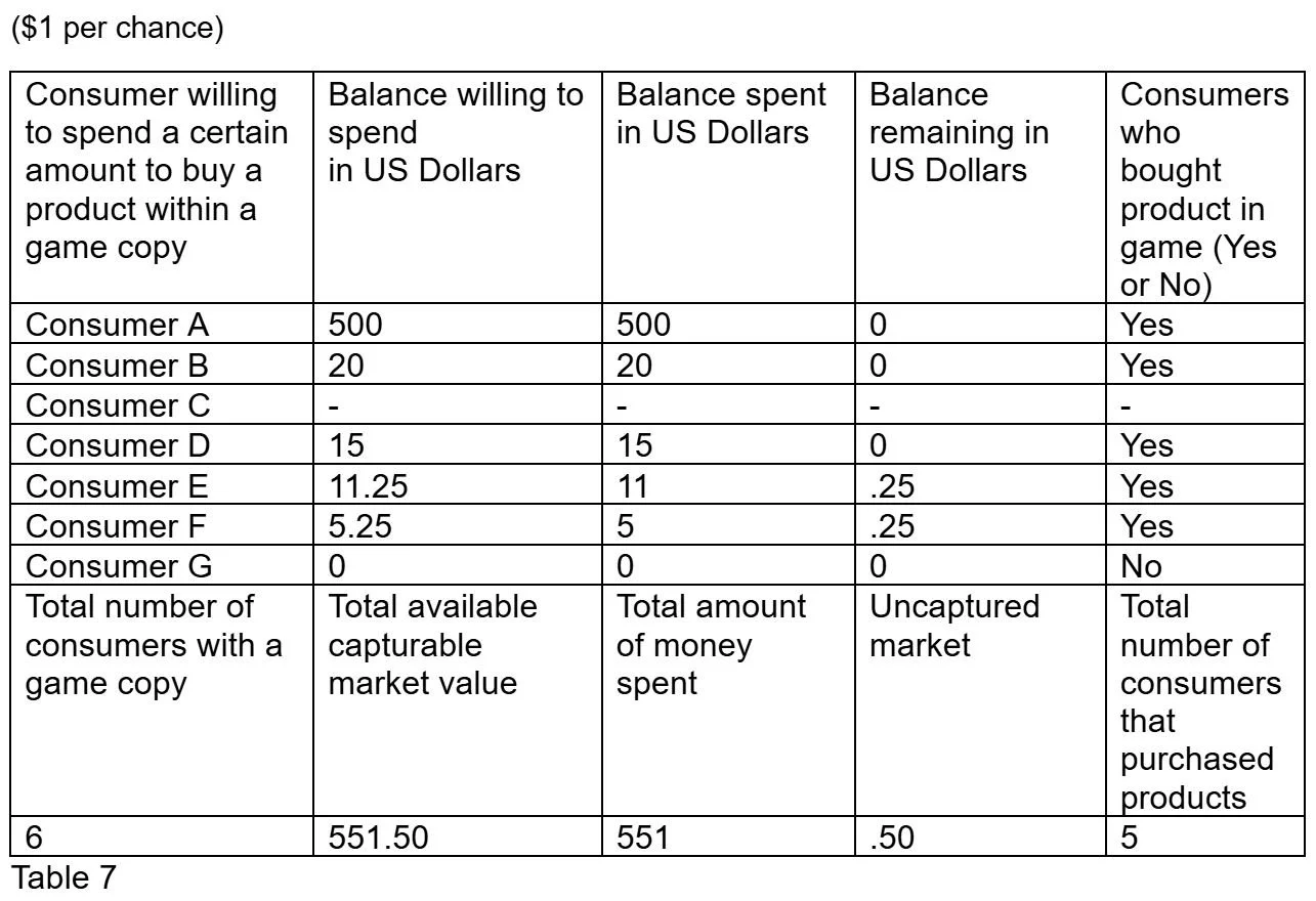
Now lets change the product to become a lottery ticket which is a roll in gacha games. Each lottery ticket costs $13 to buy and consumers can buy as many as they want within the limits of their own disposable income. Instead of a fixed price where the consumers can be guaranteed to gain a product by paying $13, customers now can pay $13 for a chance to earn a product. This is the lottery ticket. More payments like buying more lottery tickets can be done for more chances to obtain a product. Therefore, a consumer would be incentivized to pay for another chance if they did not get the product from a previous attempt of paying for a chance or chances. This behavior would occur more if the chance of obtaining a product is low compared to a product that has a high or guaranteed chance of being obtained.

Table showing $13 per chance

As shown in this table, consumers had $571.50 of disposable income and could only spend $533. All 7 consumers had a game but only 4 people could buy the product. $38.5 still remains in the hands of consumers.

Notice that the consumer who can afford multiple payments of $13 is the only type of consumer which is affected by this change from a fixed pricing system to a variable pricing system. However, the quantity of consumers who can and cannot pay a variable chance for getting the product has not changed.

This demonstrates that this change only affects inelastic consumers or people with high amounts of desire for the product and have the disposable income to buy the product. Elastic consumers or consumers that have a desire to buy the product but don’t have the funds to buy the product are not affected by this change. These consumers are shown by the complete lack of change in the total consumers who buy the product. In short, this chance sale system only gets money from consumers based on the price of each chance. If a consumer can’t afford a chance, the consumer cannot pay for the item.

So will lowering the price per chance cause consumers to spend more? Let's lower the $13 per chance to $8 per chance.

Table showing $8 per chance

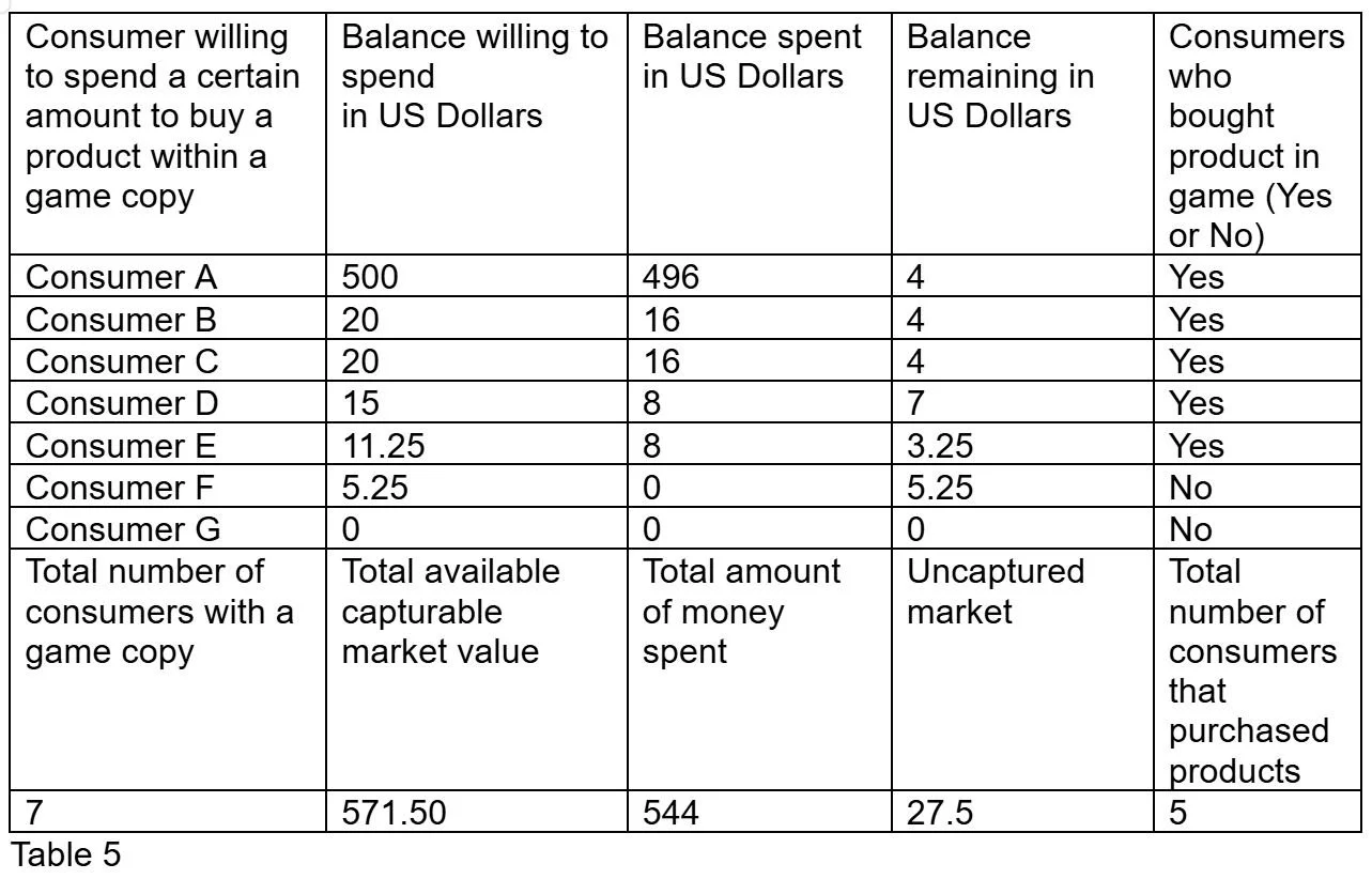
As shown in this table, consumers had $571.50 of disposable income and could only spend $544. All 7 consumers had a game but only 5 people could buy the product. $27.5 still remains in the hands of consumers.

In this example, lowering the price per chance shows that there is an increase in the dollars spent by consumers, less money remaining in the consumers, and more consumers who bought the products.  Interestingly, customers who are in the middle of the spending power range may actually spend less if the amount or rolls they can attempt do not change. This is demonstrated by Consumer D which in table 4 had spent $13 for 1 chance with $2 remaining, compare this to table 5 where Consumer D had spent $8 for 1 chance with $7 remaining. Consumer D had $15 to spend and could only spend $13 per 1 chance in table 4 while the same customer could only spend $8 per 1 chance on table 5.

Now what happens to Consumer D if the price point is lowered to $4 per chance? This can be demonstrated in the next table.

Table showing $4 per chance

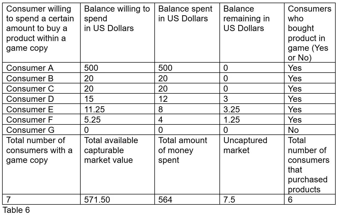
As shown in this table, consumers had $571.50 of disposable income and could only spend $564. All 7 consumers had a game but only 6 people could buy the product. $7.5 still remains in the hands of consumers.

Based on this example, Consumer D now spends $12 for 3 chances. This is lower than the $13 per 1 chance spent in table 4 while higher than the $8 per 1 chance on table 5. What this indicates is that lowering the price per chance can increase and decrease how much a consumer spends.

Since the disposable income that each consumer in the consumer group can fluctuate, it may seemingly make the sum of disposable income spent unpredictable. Now the main point of this simulation is to show the sum of disposable income spent and remaining changes at different price points for this simulated consumer group. The price points of $1, $2, $3, $4, $5, $6, $7, $8, $9, $10, $11, $12, $13, $14, $15, $16, $17, $18, $19, $20, $21, $22, and $23 per chance will be applied to each consumer group. The price points are all calculated like in table 4, 5, and 6 and the sums of disposable income spent and remaining can be placed into two different charts. Observe.

This chart shows how much disposable income remains in total per each selected price point per chance.

This chart shows how much disposable income remains in total per each selected price point per chance.

Since these charts show that it is possible to graph out and compare consumer groups across price points, additional pricing modifications can be applied to the consumer group to show changes. In this context, I want to ask four key questions.

1. What happens if a consumer with the same amount of disposable income as another consumer is removed from the consumer group? This is Consumer C and Consumer B. Consumer C will be removed for this test. 

2. What happens if a consumer with a different amount of disposable income compared to all other consumers is removed from the consumer group? Consumer D will be removed for this test. 

3. What happens if a consumer with a different amount of disposable income compared to all other consumers is reduced? Consumer D will have their disposable income of $15 be reduced to $13 for this test.

4. What happens if two effects happen at the same time? Combining question 1 and 3 together by removing a duplicate consumer and reducing the disposable income of another consumer is the main question here. This can be done by removing Consumer C and reducing the disposable income of Consumer D from $15 to $13.

To answer these questions I will show a table type for each question. To show different types of total spending and total balance remaining for each consumer group in each question, simply make another table with any of the individual chances being priced anywhere between $1-$23 (i.e question 2 but with each chance priced at $2, question 2 but with each chance priced at $3, etc…).

Question 1

($1 per chance)

Question 2

($1 per chance)

Question 3

($1 per chance)

Question 4

($1 per chance)

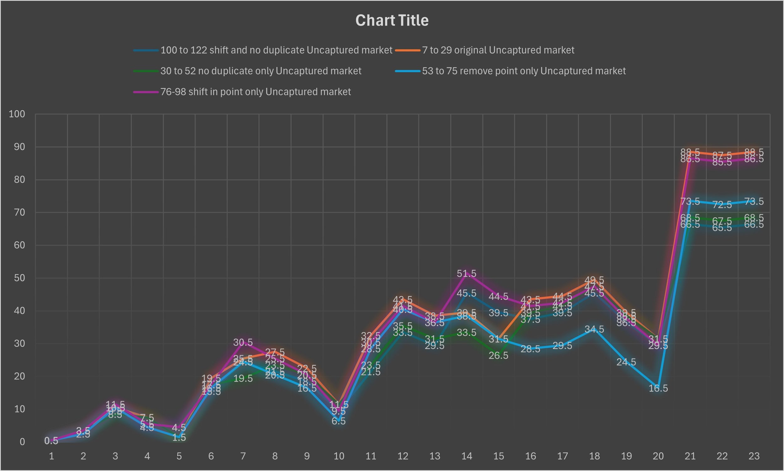
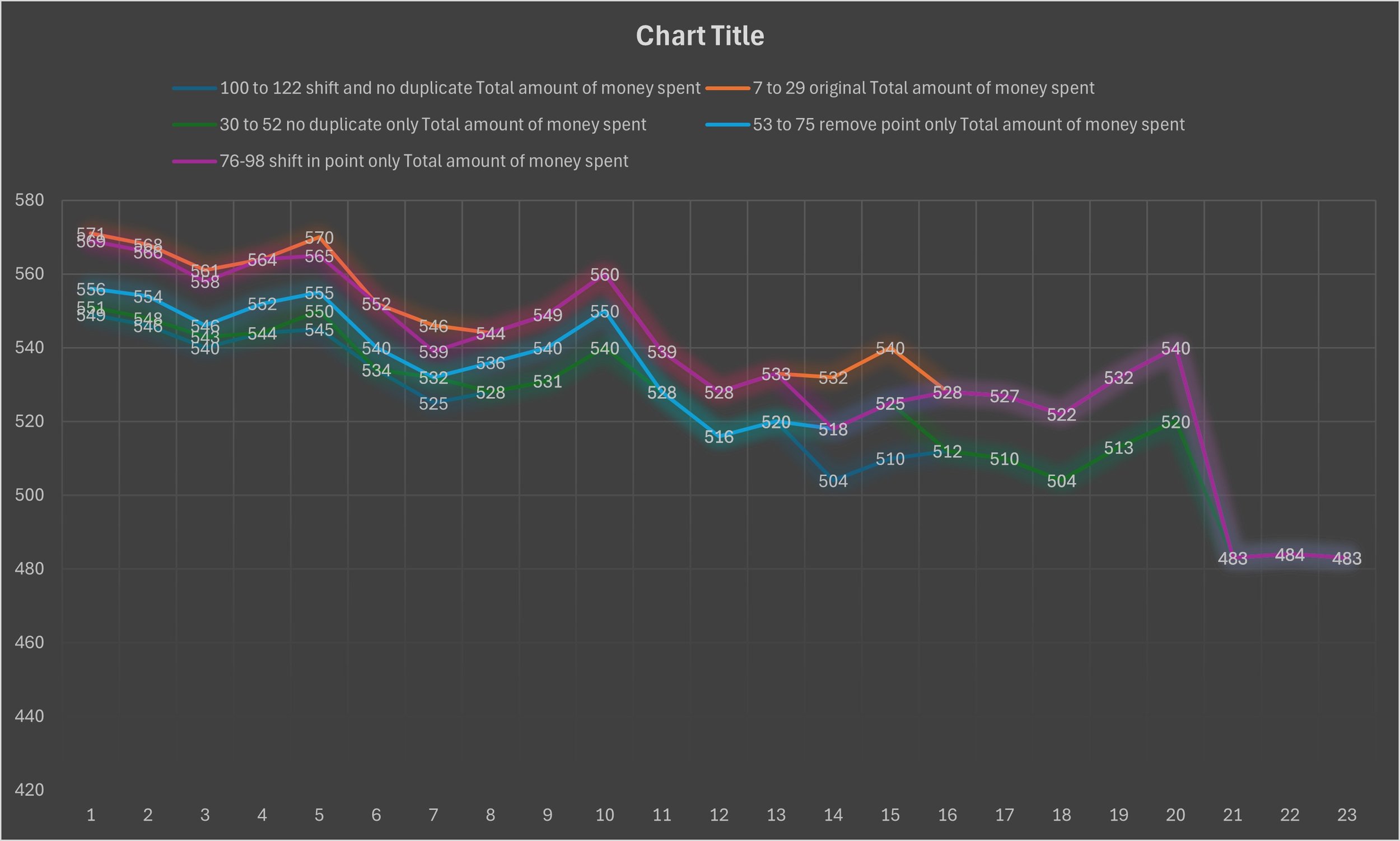
After calculating all of the tables with different prices per chance ranging between $1-$23 in whole number dollar amounts for each question. I have created a chart comparing all the questions to an unaltered consumer group. Here is a key:

7 to 29 is all combinations of $1-23 whole dollars per chance tested in an unchanged consumer group.

30 to 52 is Question 1 .

53 to 75 is Question 2.

76-98 is Question 3 .

100 to 122 is Question 4.

These two following charts show how much of the market as the consumer group is uncaptured or the total amount of money that is still in the hands of the consumer. Each total amount in the graph depends on how much each individual chance costs for the consumer.

These two following charts represent the total amount of disposable income consumers have spent. Each total amount in the chart depends on how much each individual chance costs for the consumer.

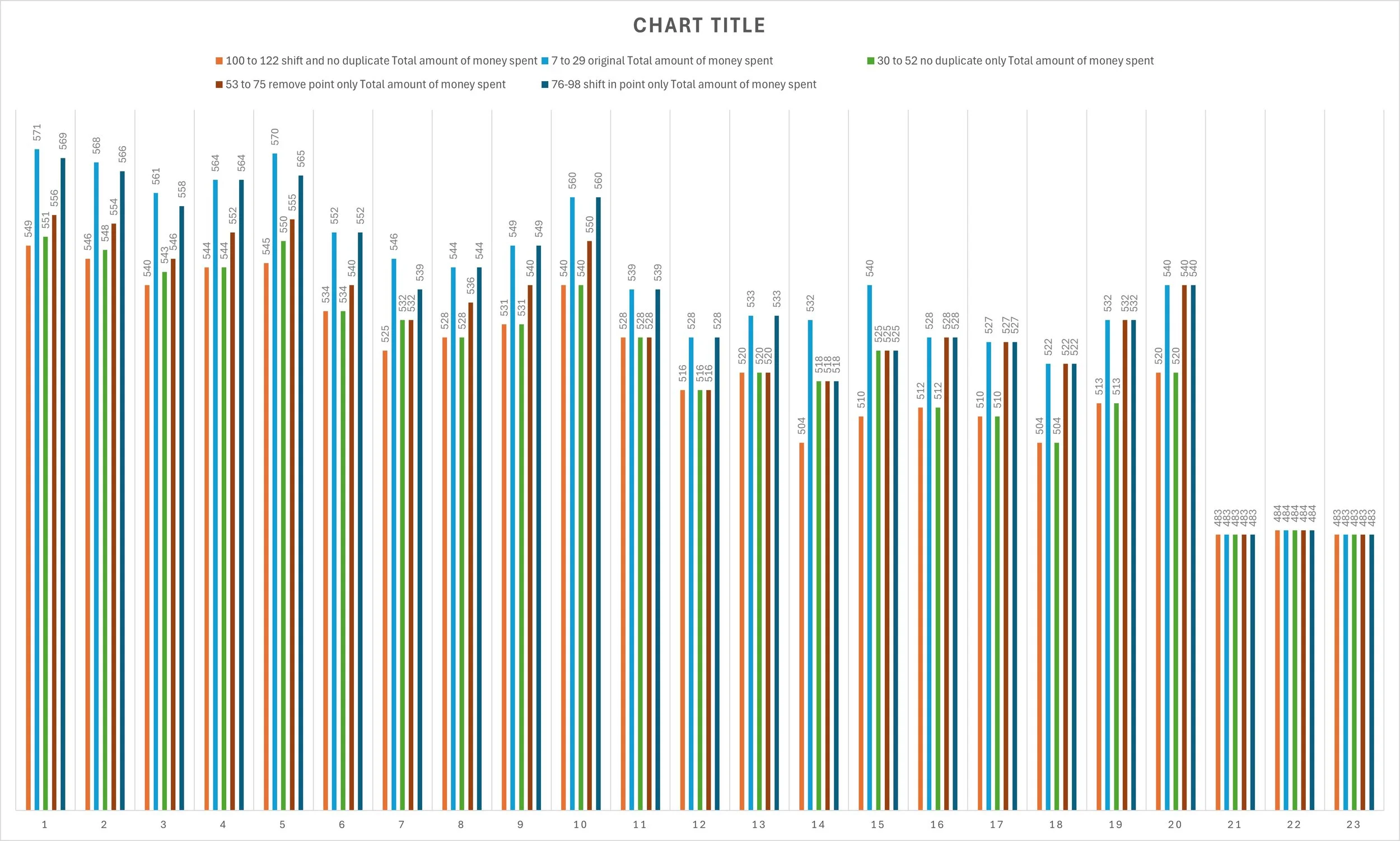
After comparing all of these charts, I have made a comprehensive table for questions 1, 2, and 3. Since question 4 adds effects together by combining questions, the conclusion that I found is that the effect is purely additive in nature. Therefore, I will only focus on questions 1 to 3 to explain what happens if the price of a chance is raised and lowered under these 3 questions.

Results of the Simulation

To simplify the results I have listed several key rules that I found when observing these consumer groups.

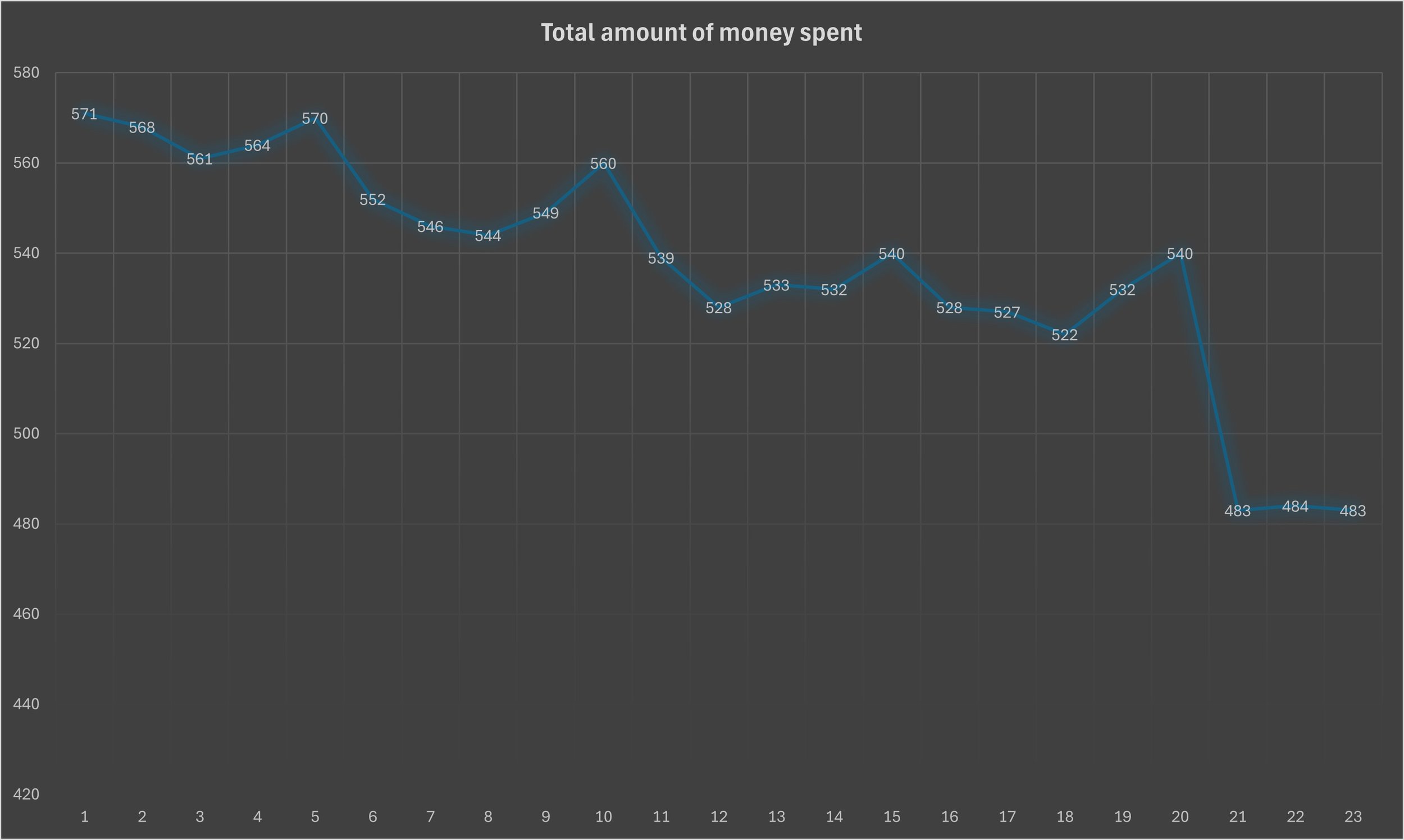
Exactly after an interval shift to a larger price point which causes a consumer to be unable to afford to pay for at least one chance, there is an increase in monetary loss guaranteed for the next one whole price point interval.

A consumer that is removed from a price point will make that price point has a loss and all less than number price points will be losses right before that price point. Observe this chart showing the removal of the only consumer at $15.

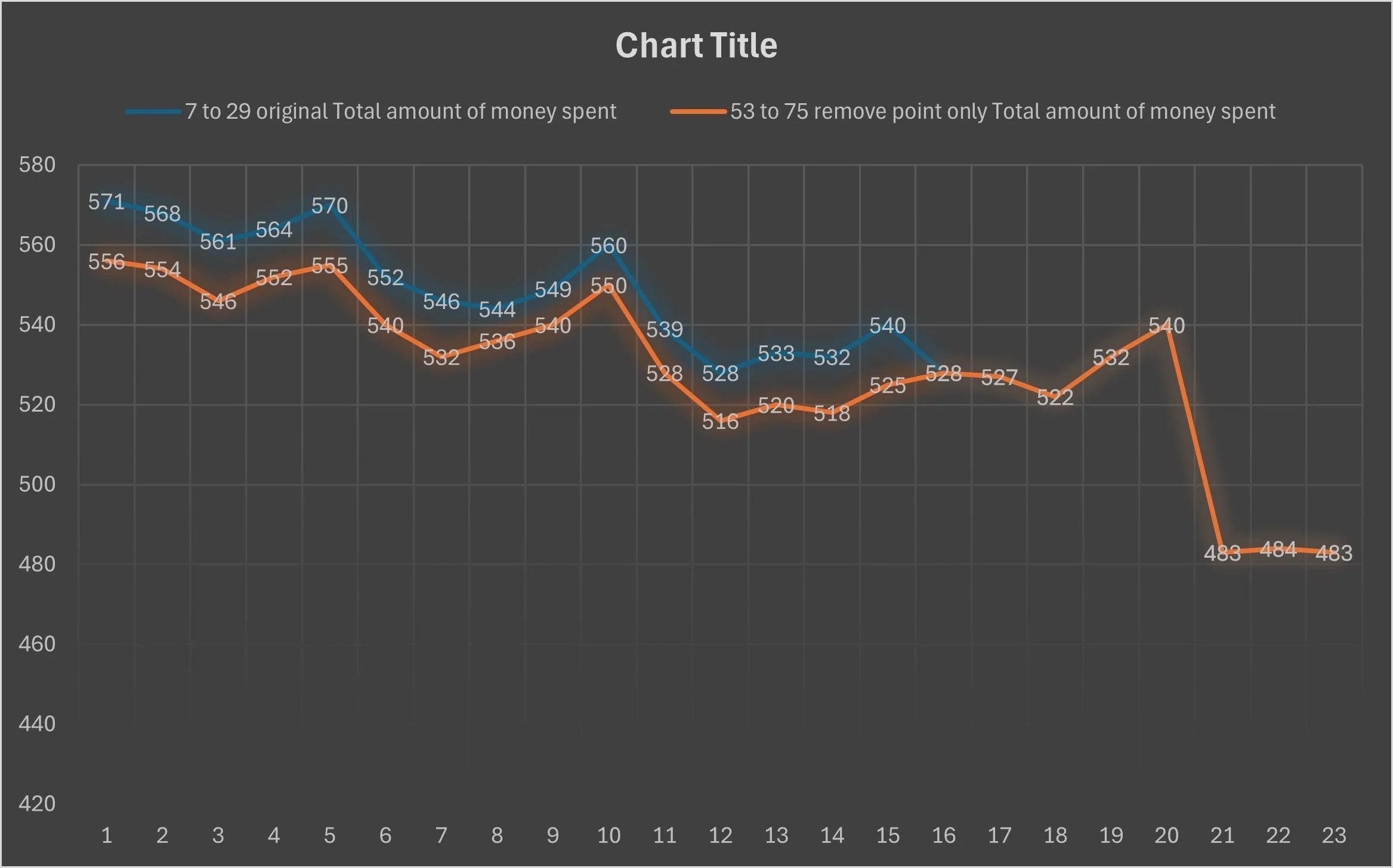
Moving a consumer from an original price point to a different price point will create losses on the original price point and can either cause no change or losses in all other price points that are only less than the original price point. Observe this chart showing the only consumer at $15 becoming $13.

In general, the smaller the price point, the more money will be made. The larger the price point, the more money will not be made.

Removal or modification of a consumer at an original price point will only decrease the money made for that original price point and smaller price points. Any consumers who are on price points bigger than the affected original price point will not be affected.

Consumers that can afford more chances who end up leaving a consumer group will negatively affect all other decisions to use lower price points to gain more money equal to and below the total spending power of the consumer that left. In short, the loss of consumers with bigger spending power will show more damage. Any damage will show at any price of a chance that is equal to or less than the disposable money of the removed consumer. 

Consumers that can afford more chances who lose spending power and shift to a lower price point may or may not negatively affect all other decisions to use lower price points to gain more money equal to and below the spending power that the consumers had before the loss of spending power. This means that there may not be damage if the consumer spends less and is not removed from the consumer group. The general key point here is that the consumer damage will be certain if the consumer is removed while there may be a chance of either damage or no damage if the consumer remains and loses spending power.

Using these points, I have created a table summarizing all the rules for when a specific scenario of a change in a consumer group (like stated in questions 1, 2, and 3) occurs and a company decision to either lower, do nothing, or change the price point relative to affected consumer spending power. “Prevent money loss” (or also called an uncaptured market) is when the video game company desires to reduce money that the consumer did not spend and “Money captured” (or also is defined as money spent by consumers towards a digital product) is portrayed as beneficial to the company. These two categories are represented in table 11.

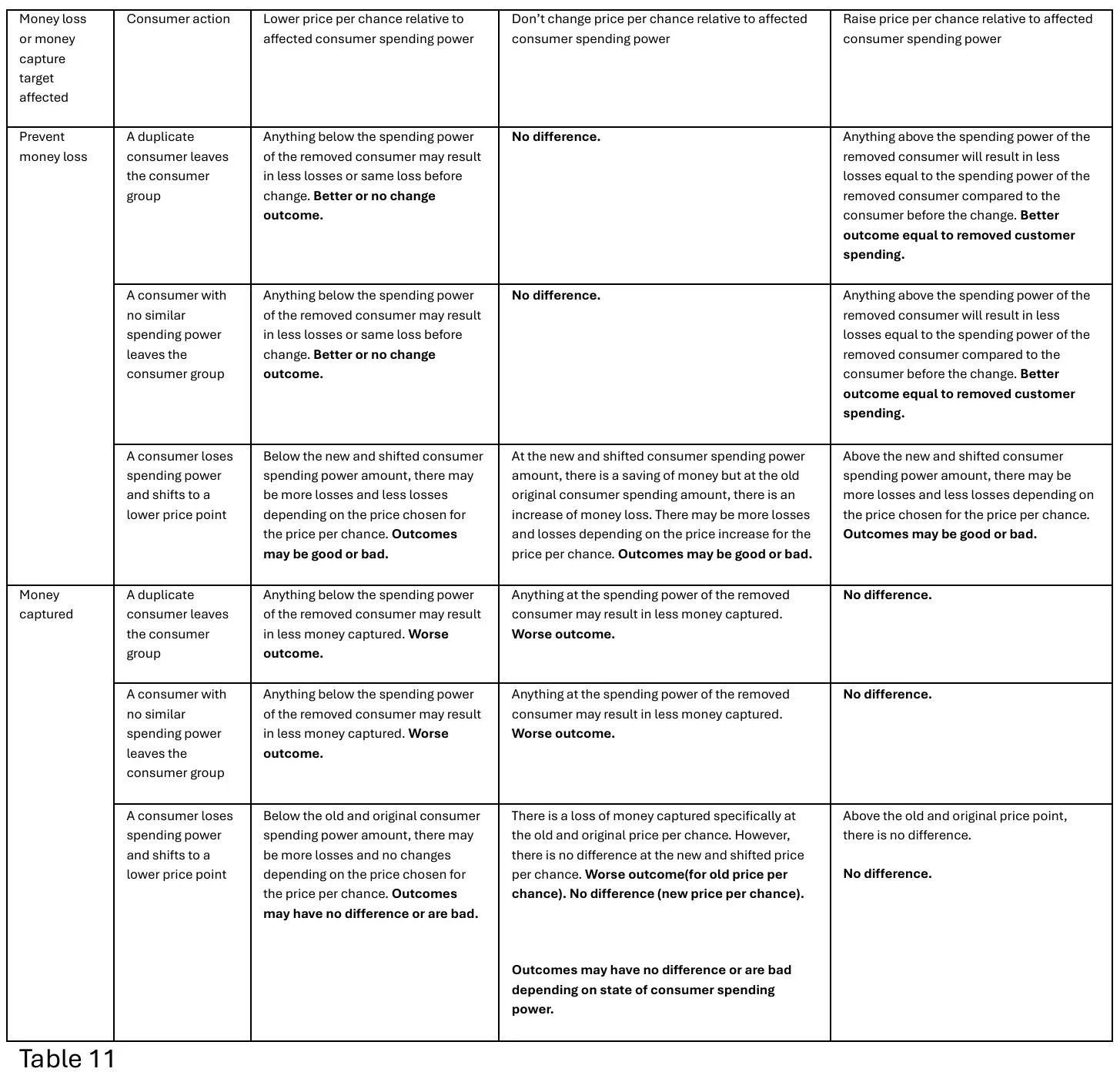
Overall, table 11 shows the possible pricing strategies that free-to-play game companies might take in response to a bout of economic downturn or changes in consumer spending if the game company has the choice to alter the price of each individual chance. Although for all simulations, the simulation shows that pricing each chance to get a product at the smallest amount will net in the most revenue. However, as consumers with spending powers begin to leave the market, monetary losses will begin to appear at any price point equal to and lower than the price point that the consumer had left in the charts that answer question 1 and 2. This is in comparison to consumers losing spending power but still paying in charts answering question 3 where points equal to and below the consumer price point before the loss of spending power have unchanged points. 

This indicates that companies are more incentivized to retain paying customers that lose spending power rather than completely lose paying customers. Based on this observation, companies will go for retaining a consumer group of hardy less spending consumers rather than consumers that can quickly default. This means that consumers with large to medium spending amounts such as wealthy consumers are prioritized for their wealth stability while consumers who can only spend a low amount are less favored due to their risk of quickly becoming unable to pay for the chance to get the digital product.  

Summary

This observation indicates that video game companies using a gacha system will naturally cater to more wealthy and stable consumers over time as more opportunities for risk will occur in the extended timeframe. Video game companies using a gacha system will advocate for a smaller denomination price per chance to capture more spending by consumers. However, if any of these companies have leeway to change their price per roll, then table 11 can show the effects of what happens to the revenue of the video game company using the gacha system. Overall, consumers will either stay in a gacha game or leave to other games depending if access to the desired digital product is available to the consumer. In the next article, I will go more into depth about what happens to consumers with different levels of disposable income that leave a gacha game.

Patreon to support the website: patreon.com/ReiCaldombra As a free member you can get notified about new uploads on Blog Under a Log. You can also become a paid member to financially support the website, but any support is greatly appreciated!

First Part: Economic Analysis on Gacha Game Pricing - Part 1 - General History — Blog Under a Log